Continuous Autoregressive Language Models
from discrete next-token prediction to continuous next-vector prediction
Introduction
Large Language Models (LLMs) represent the central paradox of modern AI. On one hand, their capabilities are unprecedented. We’ve engineered models with hundreds of billions of parameters that can synthesize vast knowledge, execute intricate reasoning, and generate everything from nuanced prose to production-ready code. In short, we’ve built Ferrari-class engines.
And yet, we’ve placed them on a narrow country road, never letting it get out of first gear. This road is the dominant paradigm of autoregressive generation: predicting text one discrete token at a time. No matter how powerful the engine, its throughput is ultimately bottlenecked by the road. This mismatch is why state-of-the-art LLMs are so inefficient and computationally expensive to run.
Historically, we have tried to widen this road by making text units larger—moving from individual characters to subword tokens. This helped, but we’ve hit the physical limits of that approach. With a typical 32K vocabulary, the semantic bandwidth of each generative step is approximately 15 bits ($\log_2 32768 = 15$). To double this bandwidth, the required vocabulary size would have to grow exponentially to $2^{30}$ entries, making the model computationally infeasible. This is the scaling wall of discrete tokens.
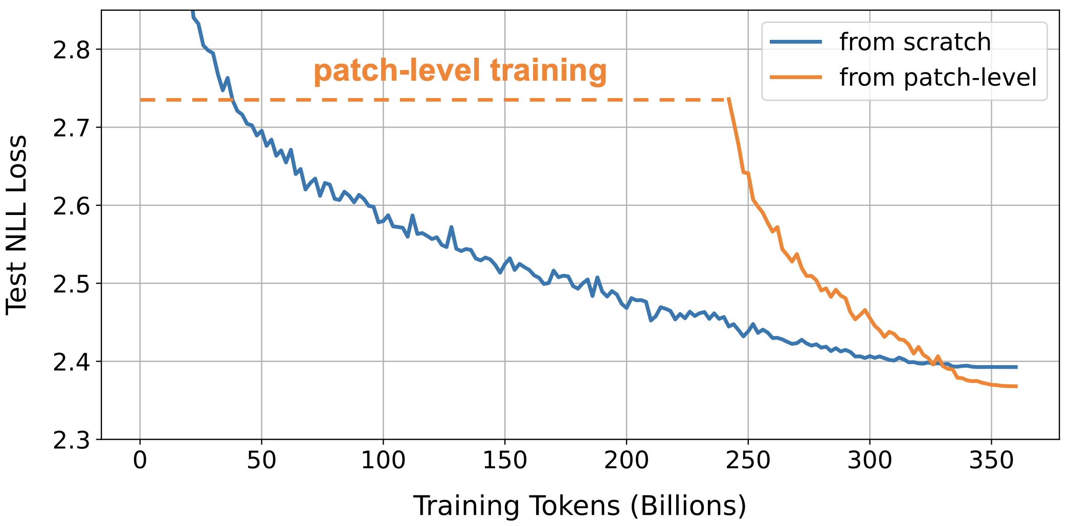
In our previous work on patch-level training, we attempted to sidestep this issue by grouping tokens into larger “patches” and training the model to predict the next patch. This allows us to process the majority of the training data at a significantly reduced cost. While this approach successfully cuts training costs by 50% without sacrificing performance, it is still constrained by the discrete nature of text. We ultimately have to fine-tune the model back to the token-level, and inference remains a token-by-token process.
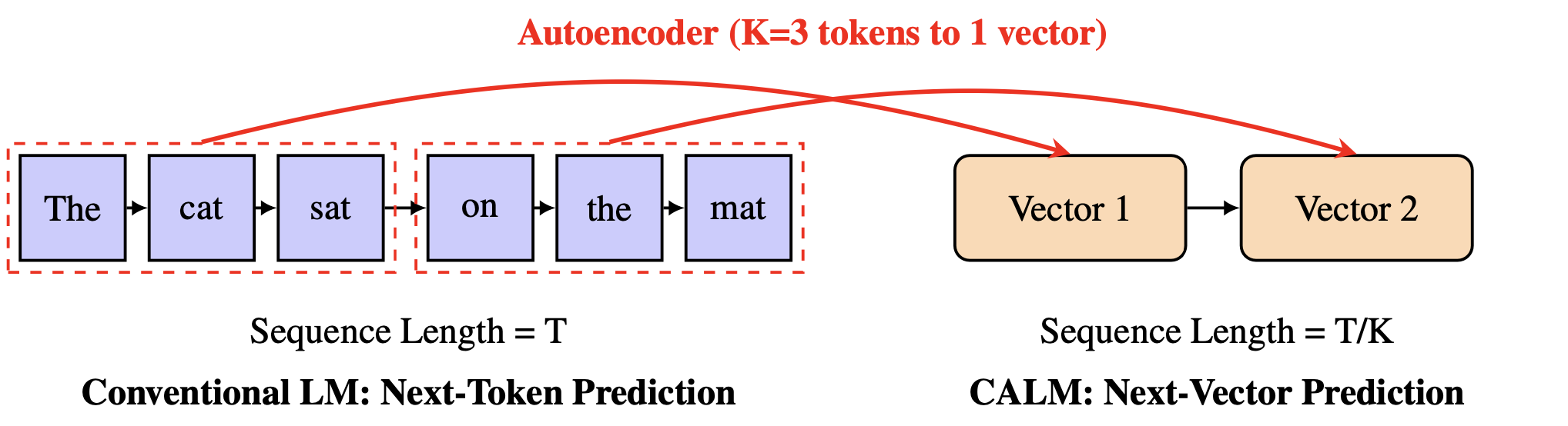
This experience makes it clear: modern LLMs possess the capacity to handle far greater information density, but the discrete token is the bottleneck. We therefore need to find a new kind of text unit with scalable semantic bandwidths. This is the core idea of Continuous Autoregressive Language Models (CALM): we shift from the discrete domain to a continuous one. Instead of predicting the next token, CALM predicts the next vector—a dense vector that represents a K-token chunk of text.
In this post, we’ll focus on the core ideas that make CALM work and omit some of the architectural details. We will cover the key challenges of modeling in a continuous space, the likelihood-free toolkit we built to solve them, and the experimental benefits of adding this new scaling axis of semantic bandwidth.
Autoencoder
The first step in building CALM is to train a high-fidelity autoencoder to establish a bidirectional mapping between discrete tokens and continuous vectors. The autoencoder is composed of two parts:
- Encoder \(f_{enc}: \mathcal{V}^K \to \mathbb{R}^l\), which takes a chunk of K tokens and compress them into a single continuous vector.
- Decoder \(g_{dec}: \mathbb{R}^l \to \mathcal{V}^K\), which takes that vector and reconstructs the original tokens.
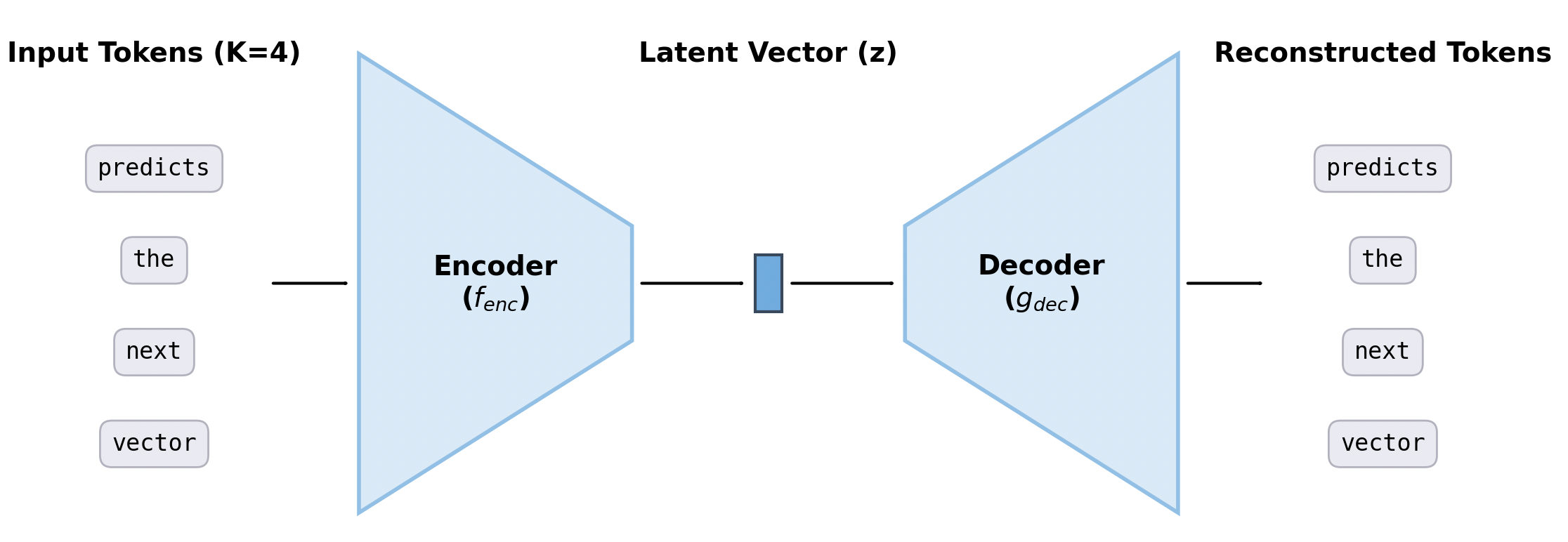
We do not delve into the specific architectures of the encoder and decoder here. They are simply composed of stacked MLP layers. The autoencoder is trained to ensure that the output tokens closely approximates the input. This is achieved by minimizing the cross-entropy loss:
\[\mathcal{L}_{\text{ae}}(\mathbf{x}_{1:K}) = - \sum_{i=1}^{K} \log p_{dec}(x_i | \mathbf{z}=f_{\text{enc}}(\mathbf{x}_{1:K}))\]For this framework to succeed, the reconstruction must be near-perfect. This is theoretically feasible when we compare the information capacity of the two representations. A discrete token contains only about 10-20 bits of information, whereas a floating-point continuous vector can store $32l$ bits. Therefore, a single vector can theoretically encapsulate the information of $K\approx 2l$ tokens through simple hard-coding. Practically, when compressing a chunk of \(K=4\) tokens into a single vector, we found that a latent vector of \(l=10\) is sufficient to achieve high-fidelity reconstruction, with a token-level accuracy of over 99.9%.
However, high reconstruction accuracy alone is insufficient for a robust generative framework, as a minor perturbation to the vector can cause the decoder to reconstruct completely unrelated tokens. To solve this, we need a smoother mapping to tolerate a certain amount of noise. Our primary strategy is to smooth the latent manifold by moving from a deterministic autoencoder to a variational one, where the encoder learns to represent tokens as a Gaussian distribution. Additionally, we incorporate dropout techniques, which force the autoencoder to learn a redundant vector representation.
The synthesis of these techniques results in a powerful and robust autoencoder. The final model maps a chunk of \(K=4\) tokens into a \(l=128\) dimensional vector. It can withstand substantial Gaussian noise of $\sigma \approx 0.3$ and still reconstruct the original tokens with over 99.9% accuracy. This lays a foundation for the subsequent learning of CALM.
Likelihood-Free Language Modeling
The autoencoder allows us to transform the original sequence of tokens into a more compact sequence of continuous vectors:
\[\mathbf{Z} = (\mathbf{z}_1, \mathbf{z}_2, \dots, \mathbf{z}_{L}), \quad \text{where} \quad \mathbf{z}_i = f_{\text{enc}}(x_{(i-1)K+1}, \dots, x_{iK})\]The model’s objective now evolves to predicting the next vector in the sequence:
\[p(\mathbf{Z})=\prod_{i=1}^{L}p(\mathbf{z}_i \mid \mathbf{z}_{\lt i})\]The shift from a discrete to a continuous domain presents a fundamental challenge. Standard language models rely on a softmax layer to compute a probability distribution over a finite vocabulary. In the continuous space, this is no longer possible, as the probability density is defined over an infinite set. This necessitates a move to likelihood-free language modeling.
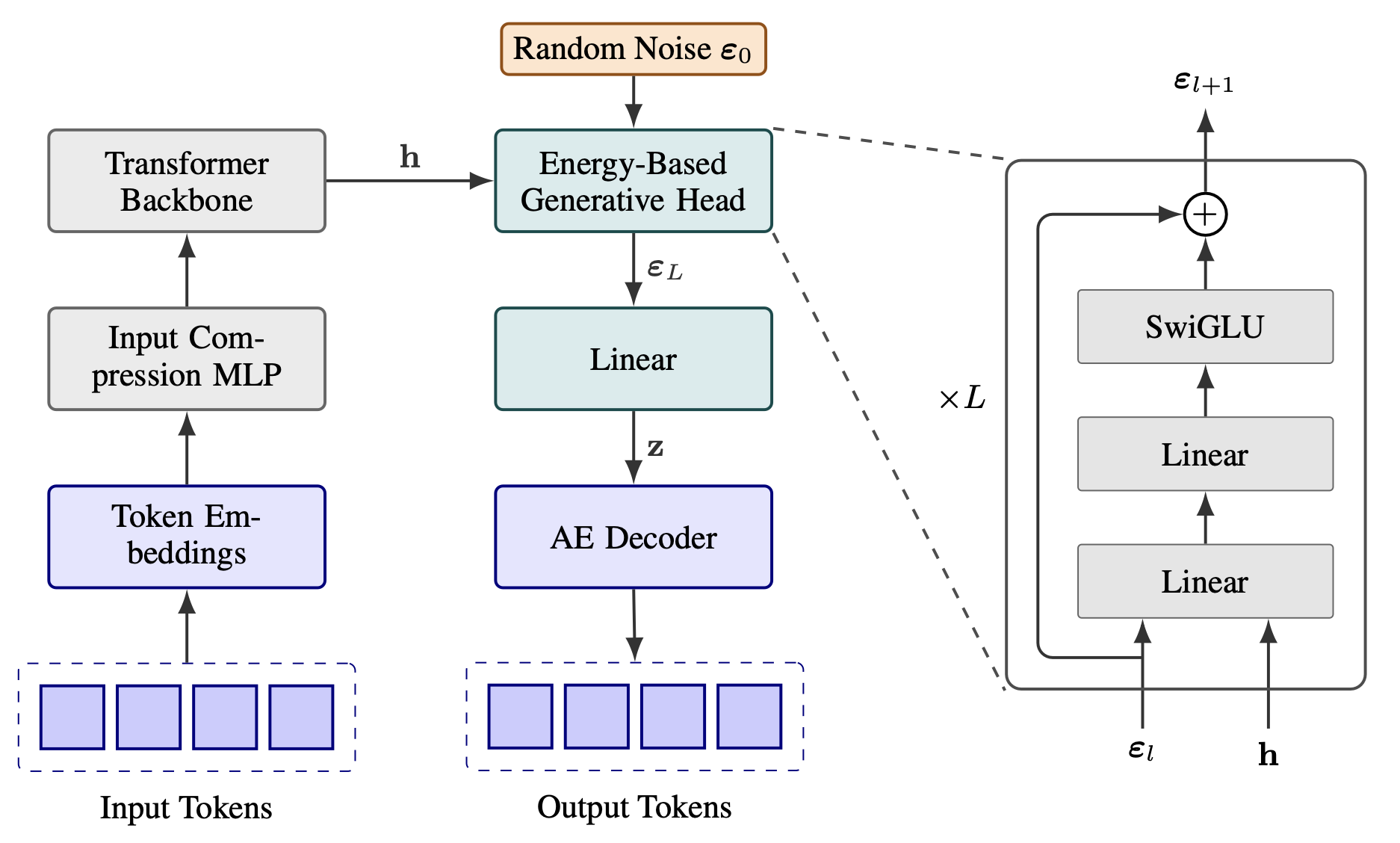
A direct approach is to find a substitute for the softmax layer that can operate in a continuous space—a component we call the generative head. Formally, the generative head is a stochastic function that takes the Transformer’s hidden state, $\mathbf{h}_{i-1} \in \mathbb{R}^d$, and draws a sample $\mathbf{z}_i \in \mathbb{R}^l$ from the conditional distribution:
\[\mathbf{h}_{i-1}=\text{Transformer}(\mathbf{z}_{1:i-1}),\quad \mathbf{z}_i \sim p(\cdot | \mathbf{h}_{i-1})\]In theory, any continuous generative model could serve as the generative head, such as Diffusion or Flow Matching. However, efficiency is critical here. Generating a single vector with diffusion requires dozens or even hundreds of sampling steps, which could counteract the speedup gained from reducing the number of autoregressive steps.
Therefore, the generative head must be capable of high-quality, single-step generation. This led us to a powerful approach based on the Energy Score. Instead of evaluating a distribution based on its probability density, the energy score assesses its quality based on the distances between samples. For a distribution $P$ and a ground truth observation $\mathbf{y}$, the energy score is defined as:
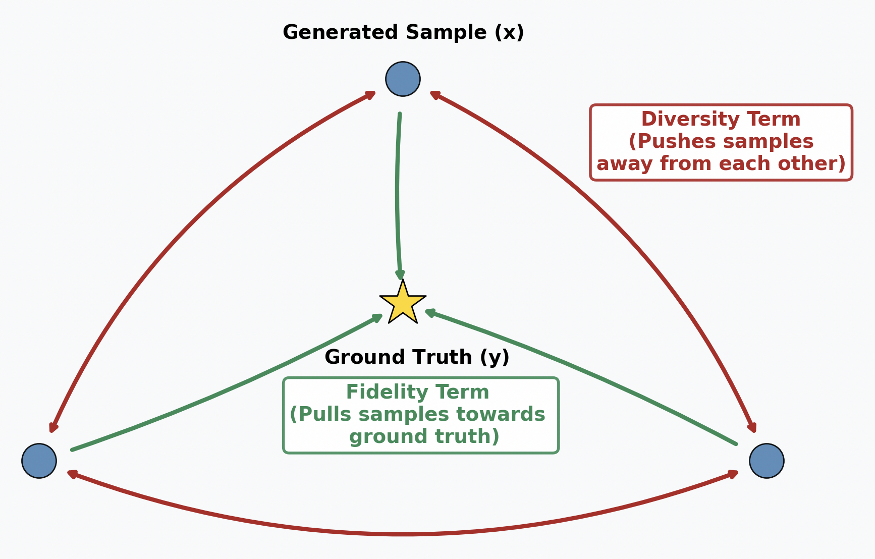
\[S(P, \mathbf{y}) = \mathbb{E}_{\mathbf{x}', \mathbf{x}'' \sim P}[\|\mathbf{x}' - \mathbf{x}''\|] - 2 \ \mathbb{E}_{\mathbf{x} \sim P}[\|\mathbf{x} - \mathbf{y}\|],\]where $\mathbf{x}$, $\mathbf{x}’$ and $\mathbf{x}’’$ are independent samples drawn from $P$. Maximizing the score forces the model to learn a balance between two competing terms:
- Diversity (\(\|\mathbf{x}' - \mathbf{x}''\|\)): This term encourages the model to generate a diverse set of samples, preventing mode collapse.
- Fidelity (\(\|\mathbf{x} - \mathbf{y}\|\)): This term rewards the model for making predictions that are close to the ground-truth $\mathbf{y}$.
The Energy Score is a strictly proper scoring rule, which means that its expectation is uniquely maximized when the model’s distribution $P$ perfectly matches the data-generating distribution $Q$:
\[\mathbb{E}_{y \sim Q}[S(P, y)] \le \mathbb{E}_{y \sim Q}[S(Q, y)], \quad \text{equality holds only when } P=Q\]In short, by training the generative head to maximize the energy score, we are implicitly driving it to learn the true data distribution. In practice, the expectations in the energy score are intractable. We instead turn it into a practical loss function through Monte Carlo estimation. At each training step, we ask the generative head to produce multiple samples, which we then use to compute an unbiased estimate of the score.
The internal architecture of the generative head is a stack of MLP blocks. To enable the model to produce different samples, we condition the generative head’s prediction on two inputs: the deterministic hidden state from the Transformer and an additional random noise vector. By drawing different noise vectors, the model can produce a diverse set of predictions from the same hidden state.
Once the generative head predicts the next vector $\mathbf{z}_i$, a natural next step would be to feed it directly as input to the Transformer for predicting $\mathbf{z}_{i+1}$. However, we found that the model struggles to unpack the semantic information from such a compact representation. Instead, we ground the autoregressive process back in the more structured discrete space, where the predicted $\mathbf{z}_i$ is passed through the autoencoder to reconstruct the K tokens. These tokens are then embedded and compressed by a input compression module before being fed into the Transformer:
Likelihood-Free LM Evaluation
Similarly, since we cannot compute explicit probabilities, the traditional perplexity-based evaluation is no longer applicable. This necessitates a likelihood-free approach to measure the model’s performance. Before introducing a new metric, it’s instructive to revisit why Perplexity is the trusted gold standard for language modeling in the first place.
Perplexity is grounded in the expected negative log-likelihood, a metric whose strength is revealed in its decomposition:
\[\mathbb{E}_{y \sim Q}[-\log P(y)] = \mathbb{E}_{y \sim Q}\left[\log \frac{Q(y)}{P(y)}\right] + \mathbb{E}_{y \sim Q}[-\log Q(y)] = \underbrace{D_{KL}(Q\|P)}_{\text{Minimized at } P=Q} + \underbrace{H(Q)}_{\text{Constant}}\]This equation is uniquely optimized when the model accurately recovers the data distribution ($P = Q$). This property encourages the model to report its true belief, as the metric cannot be hacked by a model that systematically distorts its predictions.
Under this principle, we turn to the Brier score, a classic metric that also meets this criteria. For a predictive distribution $P$ and a ground-truth outcome $y$, the Brier score is:
\[\text{Brier}(P, y) = 2P(y) - \sum_{x} P(x)^2\]It is also uniquely optimized when $P=Q$, as revealed by its decomposition:
\[\mathbb{E}_{y \sim Q}[\text{Brier}(P, y)] =-\underbrace{\sum_{x} (P(x)-Q(x))^2}_{\text{Squared Error (minimized at } P=Q\text{)}} +\underbrace{\sum_{x}Q(x)^2}_{\text{Data Variance (constant)}}\]While the Brier score is still likelihood-based, we can construct an unbiased Monte Carlo estimator using two samples from the model:
\[\text{Brier}(P, y) \approx \mathbb{I}\{x_1=y\} + \mathbb{I}\{x_2=y\} - \mathbb{I}\{x_1=x_2\}, \quad {x}_1, {x}_2 \sim P\]The first two indicator functions provide an estimate of the accuracy term, $2P(y)$. They reward the model for generating samples that match the ground truth. The third term estimates the diversity $-\sum_{x} P(x)^2$ by interpreting it as the collision probability of two independent samples.
We can apply the Brier score to assess next-token prediction performance, or we can expand its scope to measure the prediction of entire n-grams, a metric we call Brier-n. To create a single, comprehensive score, we define BrierLM as the geometric mean of the Brier-n scores for $n=1$ to $4$:
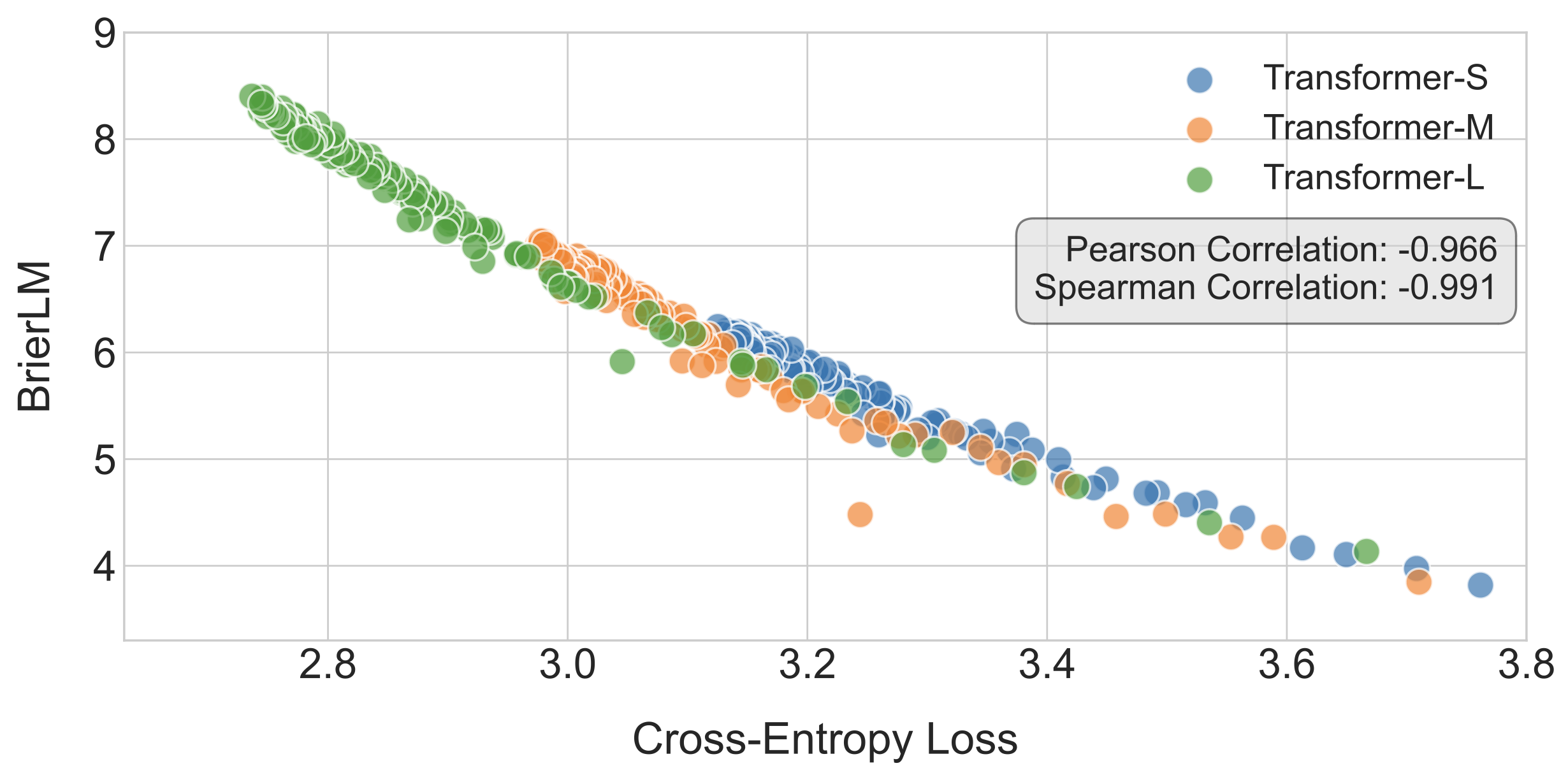
\[\text{BrierLM} = 100 \cdot \left( \prod_{n=1}^{4} \text{Brier-}n \right)^{0.25}\]BrierLM is a universal evaluation protocol that is also applicable to conventional autoregressive models. During the training of autoregressive Transformers, we observe a near-linear correlation between the BrierLM score and cross-entropy loss.
Likelihood-Free Temperature Sampling
A final challenge is temperature sampling. Users need to control the creativity of an LLM, but the standard method of dividing logits by a temperature T is unavailable to a likelihood-free model like CALM, which only gives us a sampler, not logits.
This problem can be solved with rejection sampling. Consider a simple case where we want to sample at a temperature of $T=1/n$. This is equivalent to sampling from a new distribution proportional to $P(x)^n$, the probability of drawing the same sample $x$ for $n$ times. Therefore, we can simply draw n samples from the model, and accept the result only if all n samples are identical; otherwise, we start over. For the general case, we draw upon the theory of Bernoulli Factory to construct a rejection sampling procedure with a success probability of $P(x)^{1/T}$.
A purely sequential rejection sampling approach can be inefficient. We can instead use a batch approximation: by drawing a large number of samples at once and reusing them combinatorially, the process becomes far more sample-efficient. This algorithm is asymptotically unbiased, ensuring it converges to the exact target distribution as the batch size grows.
Performance
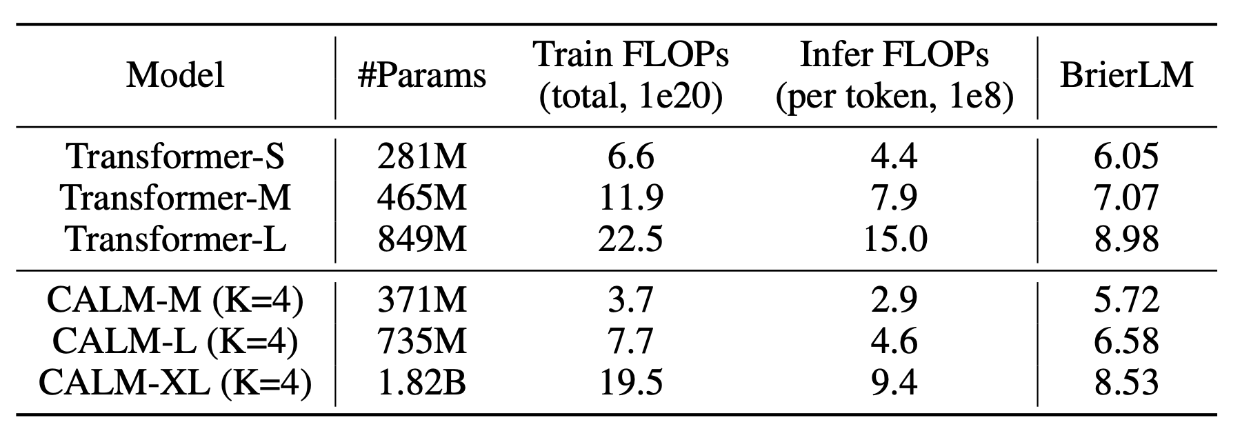
The Table below compares CALM (K=4) against traditional Transformer baselines. While a standard Transformer has stronger performance at the same parameter count, CALM requires significantly fewer FLOPs for both training and inference. This ultimately allows CALM to establish a superior performance-compute frontier.
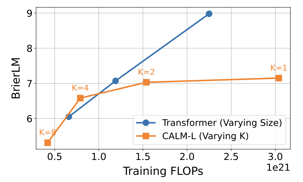
The effect of the semantic bandwidth K is shown below. At K=1, CALM’s performance lags behind its discrete counterpart, highlighting that the current design of CALM still has significant room for improvement. As we increase K, the required computation is reduced proportionally with only a marginal drop in performance. This confirms that semantic bandwidth is a highly effective scaling axis for optimizing the performance-compute of language models.
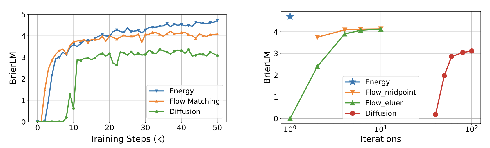
We have evaluated three kinds of generative heads: the energy-based approach, Diffusion, and Flow Matching. The diffusion model does not perform well. Flow matching exhibits faster initial convergence, whereas the energy-based head reaches a higher performance ceiling. The energy head performs generation in a single step, whereas the other two methods rely on iterative sampling. This makes the energy head a clear choice for a framework built for efficiency.
Concluding remarks
This post introduced Continuous Autoregressive Language Models (CALM), a framework that shifts generation from the discrete to the continuous domain. By using a robust autoencoder to map discrete tokens into a continuous vector, CALM unlocks a powerful new scaling axis—semantic bandwidth—to achieve a superior performance-compute trade-off.
For a detailed breakdown, please read the paper. The code is available here. Thanks for reading!